On-Premises Infrastructure and Data Center Architecture

Cloud infrastructure looks like magic until the bill arrives or a region goes down. Every EC2 instance ultimately runs on a physical server in a data center, connected by real cables to real switches, drawing real watts from a power distribution unit that ultimately traces back to a substation. When a cloud provider introduces a new instance family with higher network throughput, it is reflecting physical constraints at the hardware layer. When latency spikes without explanation, the cause often traces to a hardware decision made by the person who racked the server years ago. And when an AWS Availability Zone fails, what fails is a physical fault domain, one or more real data centers with their own power, cooling, and network fabric.

This lecture is the one place in the course that treats those physical realities as a designed system rather than as an abstraction underneath an API. It pulls together hardware concepts from the Hardware Fundamentals lecture, the addressing and ARP behavior from Networking Fundamentals, the regions and Availability Zones from the Cloud Computing lecture, and the underlay-versus-overlay framing from the Network Services and Application Delivery lecture, and answers the question those lectures kept deferring: what does the physical layer actually look like, and what decisions does it force on the people who own it?

Where Physical Infrastructure Lives

Physical infrastructure is deployed across a range of ownership and operational models. At one end, a public cloud provider (a hyperscaler like AWS, or a smaller provider like Hetzner) owns the hardware and the building; you rent capacity. At the other, your organization owns the hardware outright and may operate its own facility or place that hardware in a colocation data center where you rent only the rack space, power, and network access. Between those poles, private cloud software like OpenStack or Proxmox creates a cloud-like operations layer on top of hardware your organization owns; and the newer cloud computer approach from companies like Oxide puts a hyperscaler-style control plane on rack hardware deployed on your premises. This lecture does not weigh those business decisions. Its starting point is this: even when you choose public cloud, you are renting time on someone else’s physical infrastructure, and that infrastructure follows the same design rules as the colocation cage your competitor rented down the street.

An AWS region such as us-east-1 is not a single building. It is a geographic cluster of data centers grouped into Availability Zones, where each Availability Zone is an isolated location with independent power, cooling, and networking. AWS’s own infrastructure documentation describes an AZ as one or more discrete data centers, and AWS does not publish precise building counts. The safe operational takeaway is the one that matters: AZs are physically separated failure domains within a region, connected by high-bandwidth, low-latency regional fiber. The reason your application can survive a single-AZ outage by spreading across two or three is that those zones are deliberately separated and designed with independent power, cooling, and networking. The reason a region-wide outage is rare and catastrophic is that it usually reflects a failure in something shared across zones, such as a regional control plane, backbone dependency, or common service.

The same physics governs whether you operate the building yourself, rent space in someone else’s, or rent only the workloads. The capex-versus-opex shape of those choices is not the focus here. What matters for the rest of this lecture is that the components are the same regardless of who owns them: server hardware, storage, switches, racks, power distribution, cooling, and a network design that holds them all together.

Server Hardware at Production Scale

We already covered consumer-grade platforms: ATX boards, DDR, NVMe drives, ATX 3.x power supplies. Server hardware is a separate product line, shaped by a different set of constraints: continuous load instead of bursty workstation use, multi-socket designs, very large memory capacities, and product lifecycles measured in years rather than months. The same vocabulary applies (CPU, memory, storage, PCIe lanes), but the values and tradeoffs are different.

In vendor configurators and procurement documents, the exact sellable configuration is usually called a SKU (Stock Keeping Unit). In practice, a SKU is not just “a Dell server” or “an HPE box.” It is the specific model, CPU option, memory population, drive layout, and network configuration that can actually be ordered, racked, and supported.

Server CPUs and NUMA

The two dominant server CPU families remain AMD EPYC and Intel Xeon. Modern server parts support ECC RDIMMs (registered) and LRDIMMs (load-reduced), far more memory channels than consumer platforms, often eight to twelve per socket, and PCIe lane counts (128 or more per socket on high-end parts) that consumer chipsets cannot match. These are not “faster” CPUs in the headline sense; they are wider, with more cores, more memory bandwidth, and more I/O than a desktop part can deliver.

MZ73-LM2 Block Diagram (GIGABYTE)

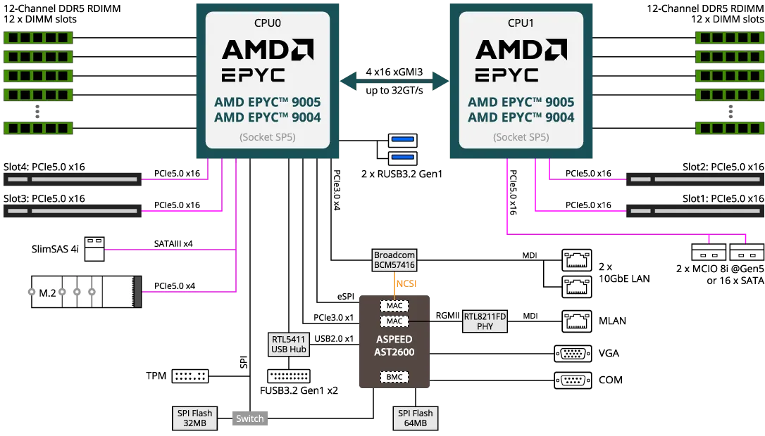
The single biggest conceptual difference for a sysadmin is Non-Uniform Memory Access (NUMA). In a two-socket server, each CPU has local memory banks it can access at full speed and remote memory banks on the other socket that it reaches over an inter-socket interconnect (AMD Infinity Fabric or Intel UPI). The latency difference between local and remote memory is typically two to three times. A workload whose threads and buffers are pinned to one socket runs at one speed; a workload whose memory ends up split across sockets runs measurably slower.

flowchart TB
  CPU0 <-->|"Infinity Fabric / UPI\n2-3x latency"| CPU1
  subgraph N0["NUMA Node 0"]
    CPU0["CPU Socket 0"]
    M0["Local DIMMs\nfast access"]
    CPU0 --- M0
  end
  subgraph N1["NUMA Node 1"]
    CPU1["CPU Socket 1"]
    M1["Local DIMMs\nfast access"]
    CPU1 --- M1
  end
  
  CPU0 -.->|"remote access"| M1
  CPU1 -.->|"remote access"| M0

Linux tools numactl and numastat expose the topology and let you pin processes and memory to a specific node. Many enterprise databases, JVM-based services, and high-throughput packet processors are NUMA-aware by default; many ordinary application servers are not, and that is the difference between predictable and surprising performance on a dual-socket node. Within a single CPU socket, modern EPYC parts also expose multiple NUMA domains per socket (NPS settings), which means even a single-socket server can have intra-socket NUMA effects worth knowing about.

ARM and AI Accelerators

For most of the modern x86 server era, “server CPU” effectively meant Intel Xeon or AMD’s server line, which today is EPYC. That is no longer a safe assumption. The hyperscalers each have an in-house ARM line aimed at general-purpose cloud workloads: Amazon Graviton, Microsoft Cobalt, and Google Axion. AWS markets Graviton as offering better price-performance than comparable x86 instances on many cloud-native Linux workloads, and porting is often as cheap as rebuilding your container for linux/arm64. Ampere Altra brings the same architecture to colocation and on-prem deployments through partners like Oracle Cloud and select OEM servers. Alongside the ARM CPUs are a generation of custom AI accelerators built for matrix multiplication rather than general compute: NVIDIA Grace Hopper superchips and GB200 rack-scale systems, Google TPU, AWS Trainium and Inferentia, and Microsoft Maia. These are not interchangeable with x86 servers; they require their own software stacks and their own networking. For this course, the operational implication is something we already touched on in the context of container orchestration: build and push multi-architecture container images so the same workload can land on whichever fleet is cheapest.

Checking Architecture in Linux

uname -m reports x86_64 on Intel or AMD and aarch64 on ARM servers. Container images must match the host architecture unless emulation (QEMU) is in play, which is significantly slower. docker buildx build --platform linux/amd64,linux/arm64 produces a multi-arch image that the registry serves to whichever architecture pulls it.

Memory at Server Scale

Building on the CPU and NUMA story, memory is where server hardware stops sounding like a faster workstation and starts becoming a reliability platform. A desktop can tolerate a little less capacity or the occasional unexplained crash. A virtualization host, database server, or in-memory cache cannot. Once a machine is holding hundreds of gigabytes or terabytes of live state, the important questions are not only how fast the DIMMs are, but how many you can populate, what kinds of faults the platform can survive, and how early the hardware can tell you a module is going bad.

ECC (Error-Correcting Code) memory stores extra check bits alongside ordinary data, and the memory controller uses those bits to detect and usually correct single-bit errors before bad data reaches the CPU. Those errors come from ordinary physics: electrical noise, cell wear, and occasionally cosmic radiation. On a laptop with 16 or 32 GB of RAM, the risk feels abstract. On a virtualization host with 512 GB or more and dozens of guest operating systems sharing the same memory pool, it stops being abstract. A single corrupted bit in page tables, kernel memory, or a live database buffer can become silent data corruption or a crash with no obvious root cause. That is why server memory treats ECC as baseline infrastructure, not as a premium option. It is also worth separating system-level ECC from the on-die error handling inside modern DDR5 chips: on-die ECC helps the DRAM chip operate reliably internally, but it does not replace end-to-end ECC that the platform can surface and log.

Capacity at server scale is also an electrical problem. Consumer platforms usually use UDIMM (Unbuffered DIMM) modules, where the memory controller drives the DRAM devices directly. As you add more DIMMs per channel, that electrical load makes clean signaling harder. RDIMM (Registered DIMM) inserts a register on the command and address path so the memory controller drives the register rather than every DRAM device directly. That buffering allows more DIMMs per channel and therefore much higher usable capacity. LRDIMM (Load-Reduced DIMM) goes further by buffering the data path as well, reducing the load seen by the memory controller even more. The tradeoff is a little more complexity, cost, and latency; the payoff is that a dual-socket server can reach multi-terabyte memory configurations that a workstation platform cannot approach.

Server platforms also add RAS (Reliability, Availability, and Serviceability) features beyond plain ECC. Memory scrubbing is the broader idea: the platform periodically or explicitly reads memory, lets ECC correct what it can, and writes corrected data back so a correctable error does not sit around long enough to become a worse one. Patrol scrubbing is the common background form. More advanced server-memory protection schemes spread data and check information across multiple DRAM devices so the system can often survive the failure of an entire memory device, not just a single flipped bit. The exact names vary by vendor and platform generation, but the idea is consistent: catch faults early, contain them, and keep one failing component from turning into bad data. That solves an integrity problem. Separate memory-encryption features solve a confidentiality problem: they protect RAM contents against physical-access attacks, but they do not repair corrupt bits. These mechanisms address different failure modes, and a well-designed server may enable both at the same time.

Operationally, memory population is not a cosmetic purchasing detail. Which slots you fill determines channel balance, achievable speed, and sometimes NUMA behavior. A DIMM that starts logging a rising count of correctable ECC errors in the BMC is giving you advance notice that replacement belongs on the maintenance schedule; an uncorrectable error is a much more serious event. Mixing UDIMM and RDIMM prevents boot, and mixing DIMMs with different rank, size, or organization can quietly force the platform to downclock or lose the balanced layout you thought you bought. Vendor population tables look tedious until the day you discover that four expensive DIMMs are running slower than two cheaper ones would have.

Server Specialization by Workload

“Server” is a generic word. Production environments use several distinct classes of hardware that look broadly similar but are optimized for different jobs.

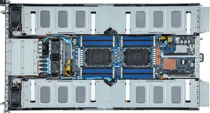
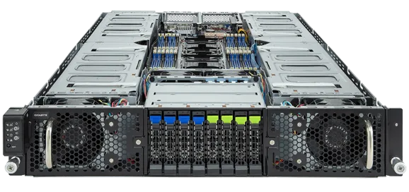
Compute and virtualization hosts are the default 1U or 2U rackmount nodes that fill most racks. A typical dense virtualization host carries one or two EPYC or Xeon sockets, several hundred gigabytes of ECC RDIMM, a small number of NVMe drives for VM images, and a 25 GbE or faster network connection. The hypervisor (ESXi, Proxmox VE, KVM, Hyper-V, or a hyperscaler’s proprietary stack) divides the box into VMs that the rest of the course already takes for granted.

Boot storage in these servers is often physically separated from the main data bays so the chassis can reserve its front-access drives for VM datastores or application data. Dell’s Boot Optimized Storage Solution (BOSS) is a representative example: a small RAID card dedicated to mirrored M.2 boot drives. Other vendors ship equivalent boot modules under different names, but the design idea is the same. Keep the operating-system mirror simple and durable, and leave the high-value front bays for data.

Storage servers invert the priorities: many drives, modest CPU and memory, and high-throughput networking. A 4U storage chassis can hold 60 to 90 spinning disks connected through a shared drive backplane, or an equivalent count of flash drives in an all-flash enclosure. The operating system is typically a storage-focused distribution: TrueNAS for ZFS-based deployments, Ceph for distributed object and block storage, or a vendor appliance OS. A JBOD (Just a Bunch of Disks) is the simplest variant: a disk shelf with no embedded compute, presenting raw drives directly to an attached server and leaving all RAID and filesystem logic to the host. The key idea is that storage hardware is often separated from compute hardware, even when the storage still looks local to the operating system.

GPU and AI servers are a different physical animal entirely. A purpose-built training node in the NVIDIA DGX class houses multiple GPUs tied together with a very fast internal interconnect such as NVLink, plus far more power delivery and cooling capacity than a normal server needs. Inference-oriented servers often use smaller accelerators because the job is serving many requests efficiently rather than training one very large model. The operational consequence is simple: once the workload spans many chassis, the network becomes part of the compute design rather than a background detail.

Head nodes or control-plane nodes are the smaller coordinating servers that sit in front of a larger cluster. In HPC and AI environments, a head node usually runs schedulers, orchestration services, login or API endpoints, service discovery, and other coordination logic rather than carrying the heavy compute load itself. That distinction matters because a cluster can need enormous aggregate GPU capacity while still needing only a small pair of head nodes.

Blade servers pack thin compute modules into a shared chassis with common power, cooling, and a networking backplane. The density is excellent and the per-node cabling drops dramatically. The tradeoff is vendor lock-in (blades from one vendor do not fit another’s chassis) and limited per-blade expansion. Blade designs were dominant in the 2000s and remain common in enterprises with long-standing HPE or Dell relationships, but most new builds use rackmount servers with top-of-rack switching instead.

Out-of-Band Management

Nearly every production server has a second computer inside it. The Baseboard Management Controller (BMC) is a small management controller, usually built around an ARM-based system-on-chip (SoC), with its own CPU, memory, and firmware that operates independently of the main CPU and OS. Many servers expose it on a dedicated management port; others can share a physical Network Interface Card (NIC) through sideband management, where the same physical port carries both host traffic and management traffic with VLAN separation. Vendor names for the BMC’s full feature set are familiar: iDRAC on Dell, iLO on HPE, XClarity Controller (XCC) on Lenovo, and CIMC on Cisco UCS. The protocol that has historically tied them together is IPMI (Intelligent Platform Management Interface), first standardized in 1998 and reaching version 2.0 in 2004; the modern HTTPS-and-JSON replacement is Redfish, which the DMTF (Distributed Management Task Force) maintains as the standard interface for new automation. Redfish was designed from the ground up for security-aware, scalable, multi-vendor server management and is now supported by all major server vendors.

Operationally, the BMC is the answer to questions that have no software-side answer. You can power-cycle a hung server when SSH is unresponsive. You can attach to the console as if you were standing in front of the rack with a monitor and keyboard, through a virtual KVM session that runs in a modern HTML5 browser without requiring Java plugins. You can mount an ISO image as a virtual CD-ROM and reinstall the operating system on a remote machine over the management network. You can read the System Event Log for hardware events the OS never saw, including the ECC errors and fan failures that signal an impending hardware problem. All of these functions work whether the host operating system is running, hung, or missing entirely, because the BMC is a separate computer that shares only power, network, and in some cases a serial console with the host.

The network design implication is the part most relevant here. The BMC presents its own management interface, with its own MAC and IP identity even when it shares cabling with a host NIC, and it should be on its own management VLAN that is reachable only from operator workstations and a small set of automation hosts. The specific VLAN number is just a local convention; what matters is that the management network is separate and tightly controlled. Putting BMCs on the same VLAN as production traffic exposes a powerful control surface to anyone who reaches that broadcast domain. A separate, firewalled, MFA-gated management VLAN is the standard pattern, and it is one of the reasons VLAN segmentation matters operationally rather than as a theoretical layer-2 nicety.

flowchart LR
  subgraph Server["Production Server"]
    OS["Host OS\napps, hypervisor"]
    BMC["BMC\nindependent SoC"]
    NIC1["Data NIC\n25 GbE"]
    NIC2["BMC NIC\n1 GbE"]
    OS --- NIC1
    BMC --- NIC2
  end
  ProdSW["Production Switch\nVLAN 10: app traffic"]
  MgmtSW["Management Switch\nExample VLAN 120: BMC only"]
  NIC1 --> ProdSW
  NIC2 --> MgmtSW
  Ops["Operator workstation\n+ automation hosts"]
  MgmtSW --- Ops
  FW["Firewall + MFA\nno public exposure"]
  Ops --- FW

BMC Security Is Not Optional

A BMC with default credentials and a routable address is one of the most direct paths to total compromise of a server: it can mount arbitrary media, capture the console, and survive an OS reinstall because it is not part of the OS. Treat BMC credentials like root credentials, keep firmware patched, and never expose the BMC interface to the public internet.

Enterprise Storage

We already covered the basics of HDD and SSD media and the M.2 NVMe drives common in consumer machines, and we introduced RAID as a concept along with ZFS and Btrfs as integrity-aware filesystems. At server and data center scale, the new questions are how drives attach (interface and form factor), how storage is delivered to consumers (locally, over the network as files, or over a fabric as blocks), and how the redundancy is organized when a single array carries dozens of terabytes that nobody wants to restore from tape.

What 'Fabric' Means

In storage and networking, a fabric is a dedicated switched interconnect that connects many servers to many storage devices. The word borrows from weaving: every node reaches the others through a shared switching pattern, like threads in cloth. A fabric differs from an ordinary LAN because it is tuned for one job, usually block storage or low-latency east-west traffic, rather than for mixed user traffic. In practice, storage teams use the word for purpose-built storage networks such as Fibre Channel, or for carefully engineered low-latency Ethernet designs dedicated to storage traffic.

Interfaces: SATA, SAS, NVMe, NVMe-oF

At storage scale, the first decision is often not filesystem but transport. Interface choice determines latency, serviceability, cabling density, and whether storage stays inside one chassis or can be disaggregated across racks. The table below compares the attachment types you are most likely to meet in current servers.

Interface	Representative throughput	Duplex	Hot-Swap	Use Case
SATA III	~600 MB/s	Half	Backplane-dependent	Budget servers, bulk storage
SAS-3 (12G)	~1,200 MB/s	Full	Yes (SAS expanders)	High-density enterprise storage
SAS-4 (24G)	~2,400 MB/s	Full	Yes	Tier-1 storage arrays
NVMe (PCIe 4.0 x4)	~7,000 MB/s	Full	Via U.2/U.3 backplane	Low-latency databases, AI
NVMe-oF	Fabric-dependent	Full	N/A	Disaggregated storage over fabric

The interesting interface-level details for a server administrator are the ones that do not appear on the desktop. SAS runs full-duplex, so it can read and write simultaneously on the same link, while SATA is half-duplex. SAS expanders allow one host bus adapter to address up to 256 drives, which is why high-density storage chassis are built on SAS rather than direct SATA. U.2 and U.3 are 2.5-inch hot-swap form factors that carry the NVMe protocol over PCIe lanes through a server backplane, giving you the throughput of M.2 NVMe with the serviceability of a SAS hot-swap bay. Hot-swap matters: pulling a drive from a running production system is normal procedure, and consumer SATA backplanes typically do not guarantee it.

NVMe over Fabrics (NVMe-oF) is the conceptual leap in the table: it takes the NVMe command set that usually talks to a local PCIe SSD and carries it across a network to remote flash. That network might be ordinary TCP/IP Ethernet, Fibre Channel (a dedicated storage networking standard), or a lower-latency transport in higher-end environments. The important point is not memorizing the transport menu. It is understanding that fast flash can be disaggregated from compute and still behave much more like block storage than like a remote file share.

Direct-Attached, Network-Attached, and Storage Area Networks

The three storage attachment models differ in where the network boundary falls relative to the storage device.

Direct-Attached Storage (DAS) is storage connected directly to a single host: internal drives, an external SAS enclosure, or a JBOD shelf. It provides the fastest access and no network overhead, but only the attached host can use it.

Network-Attached Storage (NAS) is a device or cluster that presents a filesystem over a standard TCP/IP network. The two dominant NAS protocols are NFS and SMB. NFS (Network File System), developed by Sun Microsystems, is the standard in Linux and UNIX environments; NFSv4 adds stronger identity handling and operational improvements over NFSv3, and it usually traverses firewalls more cleanly because it consolidates more behavior onto TCP port 2049. Neither version should be treated as safe on an untrusted network without extra protection such as private networking, VPNs, Kerberos, or RPC-with-TLS where supported. SMB (Server Message Block) is the standard in mixed-OS environments; SMB 3.x adds encryption and stronger authentication and is now the default file-sharing protocol on macOS and Windows. Multiple clients can mount the same NAS export simultaneously, which makes NAS the right answer for shared home directories, build artifacts, and backups.

Storage Area Networks (SANs) present raw block devices to servers over a dedicated storage path instead of exposing files over an ordinary share. In many enterprise environments that path is Fibre Channel, a purpose-built storage network with its own switches and host bus adapters. In Ethernet-centric environments it is often iSCSI, which carries older SCSI block commands over IP networks. Newer flash-heavy designs increasingly use NVMe-oF, which applies the same idea to NVMe devices. A server with a SAN-attached LUN (Logical Unit Number) sees it as a locally attached block device and formats its own filesystem on top. SANs are used in enterprise environments for databases and virtual machine datastores because they deliver low latency, high throughput, and the multipath failover behavior that NAS protocols cannot match at the same scale.

flowchart LR
  subgraph DAS["DAS: drives attached to one host"]
    DH["Host"]
    DD["Drives\n(internal / SAS shelf)"]
    DH --- DD
  end
  subgraph NAS["NAS: file access over TCP/IP"]
    NH1["Client A"]
    NH2["Client B"]
    NET1["Ethernet\nNFS / SMB"]
    NBOX["NAS appliance\nowns filesystem"]
    NH1 --- NET1
    NH2 --- NET1
    NET1 --- NBOX
  end
  subgraph SAN["SAN: block access over fabric"]
    SH1["Server A"]
    SH2["Server B"]
    FAB["Storage fabric\n(Fibre Channel, iSCSI, or NVMe-oF)"]
    SARR["Block array\nLUNs"]
    SH1 --- FAB
    SH2 --- FAB
    FAB --- SARR
  end

The diagram shows where the network boundary falls in each model. In DAS, there is no network between the host and its drives. In NAS, the network sits between the client and a filesystem that the appliance owns; clients see files. In SAN, the fabric sits between the server and raw block devices; the server owns the filesystem on top of the LUNs.

	SAN	NAS
Storage type	Block	File
Network	Fibre Channel / iSCSI	TCP/IP Ethernet
Performance	High	Moderate
Cost and complexity	High	Low
Use case	Databases, VM datastores	File shares, backups, home directories

Network storage failures have distinctive signatures that differ from ordinary connectivity failures, and the diagnostic tools are different. An NFS mount that succeeded during provisioning may go stale after a network partition: the server is reachable, the mount point exists, but read and write operations block until the kernel times out. The NFS mount options soft and hard control this: a soft mount returns an error after a timeout, which some applications handle badly, while a hard mount keeps retrying until the server returns, which is why it is the usual default for real data despite the risk of hung processes during an outage. SMB authentication failures usually manifest as “access denied” rather than a timeout, often because a Kerberos ticket expired or the client’s domain membership does not match the server’s ACL. SAN failures are more abrupt: if a Fibre Channel host bus adapter (HBA) loses zoning or an iSCSI session drops, block devices may disappear from the OS or start returning I/O errors, and filesystems on top often remount read-only or applications start failing writes to avoid corruption. The right diagnostic tools at that point are multipath -ll for multipath state and iscsiadm -m session for iSCSI sessions, not ping or dig.

RAID Levels and Integrity-Aware Filesystems

We already introduced RAID as a concept and described ZFS and Btrfs as integrity-aware alternatives. The remaining piece is the catalog of RAID levels themselves and the tradeoff between traditional RAID and modern filesystem-managed redundancy.

Level	Min. Drives	Fault Tolerance	Capacity Overhead	Read / Write Profile	Typical Use
RAID 0	2	None: any drive failure loses everything	0%	Highest read and write throughput	Scratch space, ephemeral caches
RAID 1	2	One drive per mirror	50% (with 2 drives)	Fast reads, write speed of one drive	Boot volumes, small critical pairs
RAID 5	3	One drive	One drive’s worth	Good reads, slower writes (parity calc)	General-purpose arrays (small drives)
RAID 6	4	Two drives	Two drives’ worth	Slower writes than RAID 5	Large-drive arrays where rebuilds are long
RAID 10	4	One drive per mirror pair	50%	High read and write throughput	Databases, VM datastores

RAID 6 has become the practical default over RAID 5 on modern multi-terabyte drives because the rebuild window after a single failure is long enough that a second failure during the rebuild is a realistic event. Single-parity RAID 5 on 16 TB drives is a configuration you read about in postmortems.

Software RAID such as Linux mdadm runs in the kernel and uses host CPU for parity calculations, which is cheap on modern processors and easy to move between machines. Hardware RAID offloads the same work to a dedicated controller card with battery-backed cache, which can deliver more predictable write performance but introduces vendor lock-in: a failed controller can render an array unreadable on a different model. Modern filesystems take a different approach entirely. ZFS, Btrfs, and Ceph’s BlueStore (Ceph is introduced in the next subsection) checksum every block at write time and detect silent corruption on every read, so a “RAID-Z” pool or a Ceph erasure-coded pool is not only redundant but self-healing in a way traditional RAID is not. That is why software-managed pools have largely replaced classic hardware RAID outside of specific enterprise appliances.

RAID Is Not Backup

If a RAID 1 array loses a disk and, during the rebuild, a directory is accidentally deleted, the deletion is instantly mirrored to the surviving disk. Only an external, versioned backup can restore it. Redundancy protects against hardware failure; only backups protect against everything else.

Distributed and Parallel Filesystems

Beyond the single-machine filesystems we already covered (ext4, XFS, ZFS, Btrfs), enterprise and HPC environments increasingly use filesystems that span many physical nodes. These systems trade some of the simplicity of a local filesystem for the ability to scale capacity and throughput linearly with node count, present a single namespace to many clients, and survive node failures without taking the data offline. The right way to read the rest of this subsection is on the single-node-versus-multi-node axis: ZFS and Btrfs scale up by adding disks to one server; Ceph, Lustre, IBM Storage Scale, and BeeGFS scale out by adding entire nodes.

ZFS and Btrfs, which we already discussed, are single-node integrity-aware filesystems. ZFS in particular has shaped how a generation of storage administrators think about pools, snapshots, and end-to-end checksums; it is the foundation of TrueNAS, OpenZFS on Linux, and the storage layer of many homelab and small-business NAS appliances. ZFS pools can reach multiple petabytes on a single host, but the server itself is the failure boundary: if the chassis goes down, the pool goes with it.

Ceph is the dominant open-source distributed storage system and the one worth knowing by name. It spreads data across a cluster of nodes using the CRUSH algorithm, a deterministic placement function that decides which nodes store each object without a central metadata server. The same cluster can present object storage (RGW, S3-compatible), block storage (RBD, used as backing for VM disks and Kubernetes PersistentVolumes through Rook), and file storage (CephFS). The unit that actually stores the data is the OSD (Object Storage Daemon), a Ceph process usually paired one-to-one with a physical drive or flash device. When administrators say a Ceph pool has a replication factor of 3, they mean each object is written to three different OSDs and, if the cluster is designed well, across different failure domains such as nodes or chassis. That is why a requirement for 200 TB usable at three-way replication really implies roughly 600 TB raw before headroom. When a node fails, surviving nodes rebalance the affected data automatically, so the cluster heals itself rather than requiring a human-driven rebuild. Ceph is the storage backbone underneath OpenStack, Proxmox VE clusters, and many on-prem Kubernetes deployments, and it powers some hyperscaler internal storage tiers. The operational tradeoff is complexity: a healthy Ceph cluster requires careful tuning of OSD layout, placement group counts, and network configuration, and it is not a system you stand up casually for a single workload.

GlusterFS is a simpler distributed file system that aggregates many servers’ local storage into a single namespace through a stack of translators. It was popular for shared application storage in the 2010s, but Red Hat ended commercial support for Red Hat Gluster Storage in 2024, and new deployments today more often choose Ceph or one of the parallel filesystems below.

Lustre is the parallel filesystem most associated with classical HPC. It separates metadata operations onto dedicated Metadata Servers (MDS) and bulk data operations onto Object Storage Servers (OSS), so a single large file can be striped across many storage targets and read or written in parallel by thousands of compute nodes simultaneously. Many of the top supercomputers on the TOP500 list run Lustre on their primary scratch filesystem. Lustre is built for raw throughput on highly concurrent scientific workloads; it is not a good fit for ordinary enterprise file sharing because the metadata path is optimized for a small number of very large files rather than many small ones.

IBM Storage Scale (formerly GPFS, General Parallel File System) is the proprietary equivalent at IBM, common in large enterprise HPC sites, weather forecasting, life sciences, and financial services. It supports parallel access from thousands of clients with strong POSIX semantics and integrates with IBM’s tape archive systems for hierarchical storage management, where rarely-accessed data is transparently migrated to slower, cheaper media.

BeeGFS is a newer parallel filesystem developed at the Fraunhofer Institute and now maintained by ThinkParQ. It is often chosen for smaller HPC clusters and AI training environments where Lustre is more than the team wants to operate. It scales well into the multi-petabyte range, works well with high-speed cluster networks, and has gained traction in GPU clusters where reading training datasets in parallel is the dominant I/O pattern.

Filesystem	Scale	License	Architecture	Primary Use Case	Operational Complexity
ZFS	Single node, up to multi-PB pool	Open source (CDDL)	Pooled storage with copy-on-write and checksums	NAS appliances, storage servers, homelab	Low to moderate
Ceph	Tens to thousands of nodes	Open source (LGPL)	CRUSH-placed objects; RBD, CephFS, RGW interfaces	Private cloud, Kubernetes PVs, S3-compatible object store	High
GlusterFS	Tens to hundreds of nodes	Open source (GPL)	Translator stack over local bricks	Legacy shared application storage	Moderate (declining adoption)
Lustre	Hundreds to thousands of nodes	Open source (GPL)	Separate MDS and OSS roles, striped files	Classical HPC, TOP500 supercomputers	High
IBM Storage Scale (GPFS)	Thousands of nodes	Proprietary	Parallel POSIX with HSM integration	Enterprise HPC, financial services, life sciences	High
BeeGFS	Tens to hundreds of nodes	Open source / commercial	Parallel metadata and storage targets	Smaller HPC, AI training clusters	Moderate

The decision between these is not “which is best.” It is “which one matches your workload, your operations team, and your hardware budget.” A storage server backing a few hundred home directories should probably run ZFS. A multi-tenant private cloud or a Kubernetes cluster that needs persistent volumes for many tenants should probably run Ceph. A scientific cluster reading multi-terabyte datasets into a thousand compute nodes should probably run Lustre or BeeGFS. The wrong choice does not show up at install time; it shows up six months in, when the access pattern has settled and the filesystem is asked to do something it was not designed for.

Enterprise Network Topology

We already covered the protocols (TCP/IP, ARP, DHCP DORA, NAT, routing tables) and the small-network role of managed switches, VLANs, and routers, and we extended that picture to reverse proxies, load balancers, TLS, and CNI underlay versus overlay in Kubernetes. What is left for this lecture is the topology that ties all of those things together into a network you can rack, cable, and operate.

From Three-Tier to Spine-Leaf

The Cisco hierarchical model organizes a network into three functional layers. The Access Layer is where end devices connect; it handles layer-2 switching, port security, VLAN assignment, and Power over Ethernet for things like phones and access points. The Distribution Layer aggregates access switches and acts as the boundary between layer-2 switching and layer-3 routing; it enforces ACL-based policy, performs inter-VLAN routing, and summarizes routes upward. The Core Layer is the high-speed backbone that interconnects distribution devices; it does as little policy work as possible and prioritizes fast forwarding and redundancy. In small-to-medium networks, the distribution and core layers are often collapsed into a single layer-3 switch.

flowchart TD
  Core["Core Layer\nHigh-speed backbone\nFast forwarding only"]
  D1["Distribution Layer A\nInter-VLAN routing\nACLs, route summarization"]
  D2["Distribution Layer B\nInter-VLAN routing\nACLs, route summarization"]
  A1["Access Layer\nServer VLAN 10"]
  A2["Access Layer\nUser VLAN 20"]
  A3["Access Layer\nVoIP VLAN 30"]

  Core --- D1
  Core --- D2
  D1 --- A1
  D1 --- A2
  D2 --- A3

This design is the right answer for a campus: users connect at the access layer, traffic flows up to a central core, and a small number of expensive policy points see everything. It is the wrong answer for a modern data center. Data center workloads are dominated by east-west traffic between servers: replicas in a distributed database, Kubernetes pods on different nodes, synchronization traffic between GPUs in a training cluster, or block storage traffic to a remote flash array. In a three-tier topology those flows climb to the core and back down, doubling hop count and creating oversubscription bottlenecks. Modern data centers therefore use spine-leaf (also called fat-tree or Clos) topologies instead. Every leaf switch connects to every spine switch, and no two leaf switches connect directly. Traffic that stays within one rack stays on a single leaf; traffic that leaves the rack follows a fixed, small path of leaf, spine, leaf. That gives you predictable latency between racks, and bandwidth scales by adding spines rather than upgrading a central core.

flowchart TD
  S1["Spine Switch 1"]
  S2["Spine Switch 2"]
  L1["Leaf Switch 1\nRack A"]
  L2["Leaf Switch 2\nRack B"]
  L3["Leaf Switch 3\nRack C"]

  S1 --- L1
  S1 --- L2
  S1 --- L3
  S2 --- L1
  S2 --- L2
  S2 --- L3

The oversubscription ratio is the design knob: the ratio of total downlink bandwidth (toward servers) to total uplink bandwidth (toward spines). A 4:1 ratio means four servers share one server’s worth of uplink capacity. For ordinary web and database workloads this is fine. For AI training clusters whose nodes must exchange model updates continuously, 4:1 can make a 64-GPU cluster behave more like a much smaller cluster in practice, and the right answer is a non-blocking 1:1 fabric, which is why AI cluster networking is often the most expensive line item in the rack after the GPUs themselves.

When network engineers talk about a rack’s steady-state oversubscription ratio, they mean the normal operating condition where all planned switches and uplinks are present. That is different from the degraded condition after a switch or uplink fails. A design can look comfortable in steady-state and become unacceptably tight in failure mode, which is why serious rack designs calculate both.

Historical Note From Three-Tier to Spine-Leaf

The three-tier model was designed for the traffic patterns of the 1990s and early 2000s, when most traffic flowed north-south from user desktops to central servers and out to the internet. Virtualization, distributed databases, Hadoop, and later Kubernetes flipped that pattern: most data center traffic is now east-west, server-to-server within the same building. The spine-leaf topology was not new in 2010 when it began replacing three-tier in data centers. It descends from telephony switching research published by Charles Clos in 1952. The shape of the network finally caught up with the shape of the traffic.

VLAN Operations in Practice

VLANs, which we already introduced as a way to segment a switch into multiple logical broadcast domains, take on additional operational significance at enterprise scale. The details that matter are how VLAN membership is implemented on physical ports and what happens when a port is configured wrong. Switch ports operate in one of two modes.

Access ports connect to end devices: servers, workstations, printers, IP phones. The switch assigns all traffic on an access port to a single VLAN and strips the 802.1Q tag before delivering frames to the device. The device never sees the tag. Trunk ports connect switches to each other, or switches to routers. A trunk preserves the 802.1Q tag so the receiving switch knows which VLAN each frame belongs to, which is the only way to carry multiple VLANs across a single physical cable.

flowchart LR
  Server["Server\nuntagged VLAN 10"]
  PC["Workstation\nuntagged VLAN 20"]
  SW1["Switch A"]
  SW2["Switch B"]

  Server -->|"access port\nVLAN 10, untagged"| SW1
  SW1 -->|"trunk port\n802.1Q tagged\nVLAN 10+20+30"| SW2
  SW2 -->|"access port\nVLAN 20, untagged"| PC

The most common VLAN failure mode is a patch cable moved to a port configured for a different VLAN. The server’s IP address is correct, but it is now in a broadcast domain that cannot reach the gateway. The symptom is one we already covered: ip neighbor show on the host reports the gateway entry as FAILED, because ARP resolution at layer 2 never completes. That is the diagnostic before anyone touches IP configuration. To route traffic between VLANs at all, you need a layer-3 device (a router or a layer-3 switch) with an interface or sub-interface in each VLAN. Without inter-VLAN routing, two hosts on different VLANs cannot communicate regardless of how their IP addresses are configured.

Access-Layer Hardening

A managed switch with default configuration trusts everything plugged into it. In an enterprise environment where the access ports run to rooms, conference tables, and wall jacks, that trust is unsafe. Four features together form the baseline hardening for an enterprise access layer.

DHCP snooping turns the switch into a witness for DHCP exchanges. It learns which IP address was leased to which MAC address on which port and stores that mapping in a binding table. Dynamic ARP Inspection (DAI) then uses that binding table to validate ARP packets on untrusted ports. A reply claiming that 10.0.1.1 belongs to a MAC address not in the binding table is dropped, which neutralizes ARP spoofing attacks where a malicious host on the segment tries to impersonate the default gateway. Servers with static addresses must have manual bindings added to the DAI table or their ARP traffic will also be dropped; this is one of the more common DAI rollout footguns. Port security limits how many MAC addresses a single port will learn, which prevents a rogue switch or hub from extending an access port into a multi-device fan-out. 802.1X authentication is the strongest layer: the port stays disabled until the connecting device authenticates through a RADIUS (Remote Authentication Dial-In User Service) server, a centralized authentication backend that enterprises use to enforce access policy across all switches and wireless access points. The RADIUS response can place the device into a specific VLAN. Together, these four features are the baseline configuration on enterprise access switches anywhere unauthorized devices could plug in.

DHCP Relay

DHCP starts as a broadcast, so by default a client only reaches a DHCP server on the same broadcast domain. In a network with dozens of VLANs that is not how DHCP runs: a single DHCP server cluster usually serves the whole campus, and routers or layer-3 switches act as DHCP relay agents, forwarding the broadcast as a unicast packet to the configured DHCP server and routing the response back. We already covered DORA, lease times, and the case for DHCP reservations on servers and infrastructure; relay is the operational piece that lets one server provide leases across many segments.

OSPF Inside, BGP at the Edge

Static routes work for small, stable networks. Once a network grows to multiple sites, multiple routers, or paths that may change, you need a routing protocol that exchanges reachability information automatically.

OSPF (Open Shortest Path First) is the interior routing protocol you are most likely to encounter on premises. It is a link-state protocol: each router builds a complete map of the topology, calculates shortest paths, and sends incremental updates when something changes. OSPF converges quickly after a failure and scales through its area concept, which keeps routing tables compact as the network grows. It runs on essentially every enterprise router and layer-3 switch and is what lets distribution switches in a three-tier or leaf switches in a spine-leaf learn routes from each other without manual configuration.

BGP (Border Gateway Protocol) is the routing protocol of the public internet and shows up in enterprises in three specific places. The first is multi-homing: when your organization peers with more than one ISP, BGP announces your IP block to both and lets you control routing preferences. The second is cloud connectivity: AWS Direct Connect and Azure ExpressRoute use BGP to exchange routes between your network and the cloud VPC. The third is inside Kubernetes clusters where a CNI plugin advertises pod CIDRs to the physical network through BGP rather than using an overlay encapsulation. BGP is more complex to configure than OSPF; in most on-prem environments you meet it at the edge rather than inside the campus. Link Aggregation (LAG), the 802.3ad protocol that bonds multiple physical interfaces into one logical link, remains the way you scale uplinks and add redundancy between switches and between servers and their top-of-rack switch.

The underlay-versus-overlay question (Kubernetes pod traffic riding a VXLAN encapsulation on top of the physical network, versus a BGP-speaking CNI announcing pod CIDRs into the underlay directly) is something we already covered from the Kubernetes perspective. Here it appears from the other angle: as a physical-network capability. If you do not control the physical network, BGP-based CNIs are not available to you. If you do, they can avoid the encapsulation overhead of VXLAN at the cost of pushing pod CIDRs into your routing tables.

The Data Center as a Designed System

A server in a rack is just a server. A rack full of servers, with structured cabling to a top-of-rack switch, hot/cold aisle airflow management, A/B power feeds, and a high-speed fabric tying it to the rest of the building, is infrastructure. The data center is not an accumulation of hardware; it is a deliberately designed system, and the design choices determine what kind of failures the building can survive.

Racks, Cabling, and Airflow

Standard data center racks are 42U or 48U tall, 19 inches wide internally, and either 600 or 800 mm deep. Each rack holds rackmount servers (most commonly 1U or 2U), one or two top-of-rack switches, a pair of vertical PDUs along the rear posts, and a tangle of structured cabling that should not be a tangle in a well-run facility. Structured cabling means cables are routed along defined paths in overhead trays or under raised floors, terminated in patch panels rather than directly into devices, labeled at both ends, and documented so a cable can be traced from one rack to another without unplugging anything to find out. Copper twisted-pair runs handle access links at 10 GbE or below; fiber handles spine uplinks and inter-rack runs because copper at 25 GbE and above is limited to short distances.

Airflow management is what keeps the building’s cooling investment from being wasted. Servers draw cool air through the front and exhaust hot air out the back. In a well-designed facility, racks are arranged in alternating hot aisles and cold aisles, with all server fronts facing into the cold aisle. Aisle containment uses physical barriers (ceilings, end-of-row doors, plastic curtains) to prevent the hot exhaust from one row from being inhaled as intake by the next, which keeps the temperature delta between the two aisles high and the cooling efficient. Blanking panels in empty rack units prevent hot air from recirculating through unused slots back into the cold aisle. None of this is glamorous; all of it affects the PUE (Power Usage Effectiveness) of the building, the ratio of total facility energy to IT-load energy, and therefore how much overhead you are paying on top of the IT load in what is usually the dominant operating cost category, electricity.

Top view of a dense 2U GPU server. We can see 4 GPU bays, 2 CPU sockets with 24 DIMMs (8-Channel), the serviceable drive bay in front (left), and dual PSUs in the back (right). Example: GIGABYTE G293-S41-AAP1.

Front view of a dense 2U GPU server. The front face is dominated by intake area and serviceable drives, which is why cold-aisle orientation and blanking panels matter operationally. Example: GIGABYTE G293-S41-AAP1.

Rear view of the same 2U GPU server. Redundant power supplies, management ports, high-speed I/O, and exhaust airflow all compete for limited rear-panel space, which is why structured cabling and A/B power planning are part of rack design rather than afterthoughts. Example: GIGABYTE G293-S41-AAP1.

Power: From Utility to Server

Power in a data center is delivered in multiple layers. Utility power enters the building through a transformer and switchgear, passes through Uninterruptible Power Supplies (UPSes) that bridge short outages from a battery bank, and is backed by diesel or natural-gas generators that take over for longer events once they spin up (typically within 10 to 60 seconds, covered by the UPS battery in the meantime). An Automatic Transfer Switch (ATS) sits between the utility feed, the UPS, and the generator and decides which source feeds the building at any moment.

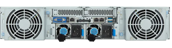
Inside the building, power is distributed to racks through PDUs (Power Distribution Units). A rack-level PDU is usually a vertical strip, and higher-end metered or switched models can report per-outlet current over the management network. Production racks almost always have two PDUs, one on each side, fed by independent branch circuits (often labeled the A feed and B feed), so a single circuit breaker trip or PDU failure does not take down the rack. Servers with dual power supplies plug one cord into each, and the supplies share load when both are healthy and carry the full load alone when one feed disappears. Sizing follows the 80 percent derating rule for continuous load, but the arithmetic depends on whether you are talking about single-phase branch power or a three-phase rack PDU. For quick mental math, single-phase nameplate capacity is roughly $V \times A$ , while three-phase nameplate capacity is roughly $V \times A \times \sqrt{3}$ . A single-phase 208 V 30 A branch circuit is about 6.2 kVA nameplate, so you plan for about 5 kW continuous load after derating. A 208 V 30 A three-phase rack PDU is a different class of feed: about 10.8 kVA nameplate, or about 8.6 kW usable continuous load after derating. At the denser end, a 415 V 60 A three-phase PDU lands around 43 kVA nameplate and about 34.5 kW usable continuous load after derating.

flowchart LR
  Utility["Utility\ngrid"]
  Gen["Diesel /\ngas generator"]
  ATS["ATS\nautomatic\ntransfer switch"]
  UPS["UPS\nbattery"]
  PDU_A["Rack PDU A\n(A feed)"]
  PDU_B["Rack PDU B\n(B feed)"]
  PSU1["Server PSU 1"]
  PSU2["Server PSU 2"]
  Server["Dual-PSU server"]

  Utility --> ATS
  Gen --> ATS
  ATS --> UPS
  UPS --> PDU_A
  UPS --> PDU_B
  PDU_A --> PSU1
  PDU_B --> PSU2
  PSU1 --> Server
  PSU2 --> Server

The redundancy story reads off the diagram: utility loss flips the ATS to the generator (with the UPS bridging the gap while the generator spins up), and a failure of either PDU still leaves the server fed by the other one. A rack that runs on only one PDU, or a server with only one power supply, is a single point of failure regardless of how good the upstream design is.

Cooling: Matched to the Load

Air cooling is the default and dominant technology for racks up to roughly 15 to 20 kW per rack. CRAC (Computer Room Air Conditioner) units use direct-expansion refrigerant loops and were the historical standard. CRAH (Computer Room Air Handler) units use chilled water from a central plant and have replaced CRACs in most new builds because chilled-water plants are more efficient at scale and easier to combine with free cooling that uses outside air when the climate allows. In-row cooling places the heat exchangers between the racks rather than at the perimeter of the room, which shortens the air path and supports higher densities. Rear-door heat exchangers mount a water-cooled coil onto the back of each rack, removing heat right where the servers exhaust it.

Above 20 to 30 kW per rack, air cooling stops being practical and liquid cooling takes over. Direct-to-chip cooling routes a water or dielectric loop through cold plates bolted to the CPU and GPU dies; the rest of the server stays air-cooled. Immersion cooling submerges entire servers in a dielectric fluid, either single-phase (the fluid is pumped through a heat exchanger) or two-phase (the fluid boils on contact with hot components and condenses on a cold plate above). Modern AI training racks routinely exceed 50 kW, and the newest rack-scale GPU systems are designed for liquid cooling from the start. NVIDIA’s GB200 NVL72, for example, is sold as a liquid-cooled rack-scale system rather than as an air-cooled retrofit. The cooling decision shapes the building: a facility designed for 8 kW racks cannot host AI workloads without renovation.

Technology	Coolant	Heat Exchange Location	Rack Density Supported	Typical Use
CRAC	Refrigerant	Room perimeter	Up to ~10 kW	Legacy data centers
CRAH	Chilled water	Room perimeter	Up to ~15 kW	Most new air-cooled builds, free-cooling friendly
In-row cooling	Chilled water	Between racks in the row	Up to ~30 kW	High-density air-cooled rows
Rear-door heat exchanger	Chilled water	Rear door of each rack	Up to ~40 kW	Per-rack densification without room redesign
Direct-to-chip liquid	Water or dielectric	Cold plate on CPU/GPU dies	40 to 100+ kW	Modern AI and HPC nodes
Single-phase immersion	Dielectric fluid	External heat exchanger	50 to 150+ kW	Crypto, HPC, dense GPU clusters
Two-phase immersion	Boiling dielectric fluid	Condenser above the tank	100+ kW	Bleeding-edge AI, research deployments

Tier Classification

The Uptime Institute publishes a four-tier classification that sets vocabulary for data center reliability.

Tier	Annual Availability	Redundancy	Concurrently Maintainable	Fault Tolerant	Typical Use
Tier I	~99.671% (~29 hr downtime/yr)	None (N)	No	No	Small business server rooms
Tier II	~99.741% (~22 hr/yr)	Redundant components (N+1) on a single path	No	No	Small enterprise
Tier III	~99.982% (~1.6 hr/yr)	N+1 with multiple distribution paths (one active)	Yes	No	Enterprise, most colo deployments
Tier IV	~99.995% (~26 min/yr)	2N active power and cooling	Yes	Yes	Banks, government, critical national infrastructure

Tier III is the practical baseline for serious enterprise and colocation deployments. Tier IV is rare and expensive; most hyperscaler data centers are not classified by Uptime at all because hyperscalers prefer to handle redundancy at the application layer across multiple Availability Zones rather than paying for fault tolerance within a single building.

High-Speed Fabric

Consumer and small office equipment still commonly operates at 1 GbE. Servers and storage have moved well beyond that.

Speed	Common Use
10 GbE	Legacy server uplinks, storage replication, older deployments
25 GbE	Standard modern server NIC in new builds
40 GbE	Older aggregation; largely replaced by 100 GbE
100 GbE	Top-of-rack uplinks, storage servers, GPU cluster nodes
400 GbE	Spine switches, hyperscale core, AI cluster interconnects
800 GbE / 1.6 TbE	Emerging standards for next-generation AI clusters

A modern compute server often ships with a dual-port 25 GbE NIC for data traffic and a separate management port for the BMC VLAN. A storage or AI server scales up: dual-port 100 GbE is common, and the AI nodes go to 400 GbE per port with multiple ports per chassis.

Ordinary Ethernet networking already uses DMA, but the host CPU and kernel still do most of the protocol work and data often traverses more of the software stack than dense storage and HPC workloads want. Remote Direct Memory Access (RDMA) lets a NIC place data directly into remote host memory with far less CPU involvement, which reduces both latency and CPU overhead. Two families matter here. InfiniBand is a dedicated high-performance interconnect common in classical supercomputing and in some of the largest AI clusters. RoCE (RDMA over Converged Ethernet) brings the same basic model to Ethernet hardware. The operational point is simpler than the acronyms suggest: when storage nodes or GPU workers must exchange large amounts of data continuously, cutting protocol overhead can determine whether the cluster scales cleanly or stalls under its own traffic.

RoCE has an important catch: the Ethernet fabric has to behave close to losslessly for that traffic class. In practice, lossless behavior does not mean the entire network literally never drops a packet. It means the switches and NICs are configured so RoCE traffic avoids ordinary best-effort packet loss, typically through tools such as Priority Flow Control (PFC) and Explicit Congestion Notification (ECN). NVIDIA’s RoCE documentation is explicit here: RoCE “requires a form of flow control” and the normal approach is PFC across the full path. If you enable RoCE on a fabric that treats it like ordinary best-effort traffic, latency and tail behavior become much less predictable.

A SmartNIC is a NIC with embedded processors or programmable packet-processing logic. A DPU (Data Processing Unit) extends that into a complete system-on-chip that runs its own operating system alongside its network processing. NVIDIA BlueField, Intel IPU, and AWS Nitro all reflect the same architectural move: push infrastructure work such as overlay encapsulation, storage encryption, firewalling, virtual switching, and telemetry off the host CPU and into dedicated hardware. From the rack’s perspective, the DPU is the point where work that once lived in the hypervisor or the host kernel starts migrating into the network card itself.

AI Cluster Network Design

A distributed training job on 64 GPUs runs an all-reduce, a collective operation that exchanges and combines gradients across the cluster, after each batch. If the fabric is oversubscribed 4:1, that synchronization step can spend more time waiting on bandwidth than computing, and your expensive 64-GPU cluster behaves more like a much smaller one. A non-blocking high-speed fabric removes that bottleneck. This is why AI cluster networking is often the second-largest line item in the rack after the GPUs themselves.

Takeaways

The physical layer is not a separate subject from the rest of this course. It is the substrate that every other layer rides on, and once you can see it, the abstractions higher up read differently. An EC2 instance type is a slice of a specific server, plugged into a specific top-of-rack switch, in a specific rack, in a specific Availability Zone. The reason r5n.large and m5.large have different network performance reflects differences in the host platform, Nitro offload path, and how much network bandwidth AWS allocates to that instance size, all of which still roll up to real rack and fabric capacity. When a region outage hits the news, it often traces to a shared control-plane, network, or dependency failure at this layer: a BGP misconfiguration, a routing-table change, or a DNS dependency that turned out to be co-located with the systems it was supposed to direct traffic to. The physics underneath the API is not exotic; it is the rack you read about in this lecture.

On-premises operations make those same constraints unavoidable rather than invisible. A disaggregated storage design built on NVMe-oF often needs very fast networking, commonly 100 GbE or better and sometimes a lower-overhead transport, or the flash tier stops behaving like flash from the application’s point of view. An AI training cluster with 64 GPUs requires a non-blocking spine-leaf fabric or its cross-node synchronization step will serialize on an oversubscribed uplink. A VLAN that segregates BMC management traffic from production data is the difference between a hardening exercise and an unrecoverable compromise. A pair of independent PDU feeds and dual-supply servers is the difference between “one breaker tripped” and “the rack went dark.” Tier III concurrent maintainability is the difference between scheduled maintenance and a planned outage.

The hardware itself has grown more varied, not less. EPYC and Xeon are still the defaults, but ARM in the cloud (Graviton, Cobalt, Axion) and Ampere on premises have become real options for cloud-native workloads, and the AI accelerators (Trainium, Inferentia, TPU, Grace Hopper) sit on top of all of this as a category of hardware purpose-built for one class of computation. The job has not gotten simpler. What has changed is that the operator who can read across layers (from the rack power budget to the spine uplink to the NUMA topology of the host to the Kubernetes scheduler) is the one who can decide whether a problem actually lives where the alert says it does. That cross-layer reading is what this lecture, and the rest of the course, is ultimately preparing you to do.

Resources

• A DAY in the LIFE of the DATA CENTRE | RACKING SERVERS with ASH & JAMES! (Custodian Data Centres) (YouTube)
• The history of servers, the cloud, and what’s next, with Oxide Computer (The Pragmatic Engineer Podcast) (YouTube)
• AWS Data Centers (AWS)
• Cisco CCNA Training Series (Network Direction) (YouTube)